Give each method a specific job, compare like with like and keep the uncertainty visible.
Physics, order of magnitude, bounds
Manufactured geometry and real fluid behaviour
Local fields, flow split and detailed comparison
A pressure-drop prediction often begins with a deceptively simple request: “Tell us how much pressure this system will lose at the required flow.”
The arithmetic may be straightforward for a long pipe. The real installation may also contain reducers, valves, manifolds, short disturbed runs, uncertain internal diameters, temperature-sensitive viscosity and equipment for which no reliable loss coefficient exists. One neat answer can therefore conceal several different questions.
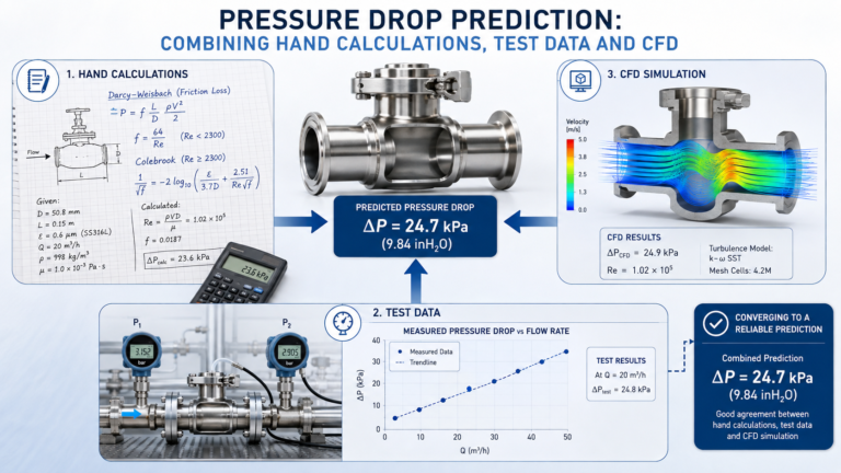
Hand calculations, physical testing and Computational Fluid Dynamics (CFD) each reveal something useful. None should automatically be treated as the senior method. The defensible approach is to give each tool a specific job, compare their outputs and retain the uncertainty that remains.
Hand calculation
Exposes governing relationships and sensitivity to uncertain inputs.
Test data
Anchors prediction to the actual component, rig and fluid.
CFD
Resolves the local geometry and mechanisms that one-dimensional models miss.
Define the pressure-drop question first
Pressure drop is not meaningful without a defined system boundary and operating condition. Before selecting a method, record:
- the inlet and outlet measurement or calculation planes;
- whether static, dynamic or total pressure is required;
- volumetric or mass flow and its reference condition;
- fluid composition, density, viscosity and temperature;
- pipe internal diameters, lengths, elevations and roughness;
- valve positions and equipment operating states;
- whether the duty is steady, pulsating or transient;
- the decision the result must support.
This matters because three apparently similar tasks demand different evidence:
- Concept screening: Is one arrangement likely to have materially less loss than another?
- System sizing: What pressure must the pump or fan provide across an operating range?
- Acceptance: Does manufactured equipment meet a specified pressure-drop limit?
The first may tolerate bounded simplifications. The third normally needs traceable test conditions, an agreed measurement method and an uncertainty statement. NASA’s validation guidance similarly treats validation as application-specific, based on comparison with experimental data over a relevant range, rather than as a permanent certificate for a CFD code.[1]
Relative difference
Bounded simplifications may be enough to separate concepts.
Operating range
Estimate the pressure source required across credible duties.
Traceable evidence
Requires agreed conditions, method, limits and uncertainty.
Use hand calculations to establish the physics and bounds
For a single-phase Newtonian fluid in a reasonably conventional pipe system, a useful first estimate is:
where:
- Δp is the predicted pressure loss;
- f is the Darcy friction factor;
- L is straight-pipe length;
- D is internal diameter;
- ρ is fluid density;
- v is mean velocity;
- K is a local loss coefficient.
The equation separates distributed pipe friction from local losses, but it does not decide whether the selected values represent the installation. That remains engineering work.
What the hand calculation should do
A good first model should:
- establish the expected order of magnitude;
- expose which dimensions and properties dominate;
- show how loss changes with flow;
- identify missing or weak input data;
- provide upper and lower bounds where inputs are uncertain;
- create an independent check for test and CFD results.
Do not hide uncertain inputs behind excessive decimal places. If the actual bore, roughness or hot-product viscosity is unknown, calculate credible cases and state what would change the decision.
Where the simple model becomes weak
Published or estimated loss coefficients may become unreliable when fittings interact, upstream flow is strongly disturbed, a valve is partly open, geometry differs from the reference configuration, or non-Newtonian behaviour makes viscosity dependent on shear rate. A one-dimensional total can also miss maldistribution, separation and recirculation.
Those weaknesses do not make the calculation useless. They show where measurement or a spatial model could add evidence.
Treat test data as measured evidence, not unquestionable truth
A pressure-drop test connects the prediction to manufactured geometry and real fluid behaviour. It can also contain its own errors.
NASA notes that experimental datasets contain bias and random errors which should be quantified and documented when they are used for validation.[1] NIST’s liquid-flow calibration practice uses controlled pressure and temperature, a developed flow profile, repeated measurements and stated uncertainty rather than relying on one indicated value.[4]
Minimum useful test definition
For a component or assembly, record at least:
- test article identity, revision and internal condition;
- fluid and measured temperature;
- fluid-property source or measured viscosity;
- flowmeter, pressure instruments and calibration status;
- pressure tapping positions and geometry;
- upstream and downstream pipe arrangement;
- flow set points, settling rule and repeat count;
- raw readings, zero checks and data-reduction method;
- estimated measurement uncertainty.
Pressure taps placed inside a local disturbance can produce a result that is repeatable but poorly representative of the intended boundary. Instrument range matters as well. A differential-pressure transmitter selected for the highest-flow point may resolve the lowest-flow point badly.
One test point is better than none, but several points across the operating range are more informative. They reveal the shape of the loss curve and may expose a regime change, instrumentation offset or an incorrect fluid-property assumption.
Repeatable can still be wrong
Pressure taps inside a disturbance may repeatedly measure something different from the intended boundary. Instrument range and low-end resolution matter too.
Use CFD where local geometry controls the loss
CFD can be valuable when the pressure loss depends on three-dimensional passages, interacting bends, manifolds, valve openings, jets or separated regions that cannot be represented confidently by standard coefficients.
It can provide:
- pressure and velocity fields;
- component-by-component loss distribution;
- branch flow split;
- recirculation and separation locations;
- consistent comparisons between design variants;
- sensitivity to selected operating or geometric changes.
However, CFD introduces physical-modelling, discretisation, iterative and usage errors. A converged solver does not remove those categories.[2] NIST identifies model quality, analyst understanding, verification, validation and uncertainty quantification as fundamental contributors to credible industrial CFD.[3]
Where CFD earns its effort
Three-dimensional passages, interacting bends, manifolds, valve openings, jets, separation and branch flow split.
Keep the CFD domain focused but connected to the system
There is little value in meshing metres of ordinary straight pipe if the real question concerns a compact valve or manifold. Model the region where spatial behaviour matters, then represent the wider system with justified boundary conditions or a simpler network model.
Published OpenFOAM work demonstrates this combined idea by using an extended Bernoulli-based boundary condition to represent external hydraulic-system losses around a detailed component domain, with the implementation checked against experimental data.[5] This does not make that exact method universal, but it shows why one-dimensional system behaviour and local CFD need not be competing approaches.
For pressure-drop work, define averaging planes away from immediate disturbances where practicable. Check mass conservation, monitored pressure difference, residual behaviour and sensitivity to mesh refinement. Where wall treatment or turbulence modelling can affect separation and friction, state the choices and their limitations.
Build one evidence chain instead of three disconnected answers
The strongest workflow is iterative.
Mark the physical endpoints, elevations, instruments, straight lengths and the detailed component. Agree what pressure quantity is being compared.
Calculate the straight-pipe and known local losses. Run sensitivity cases for uncertain bore, roughness, viscosity and coefficients. Record the expected pressure-drop band.
Choose flow points that cover the intended duty and any suspected transition. Place instruments so that the measurements correspond to the calculation and CFD planes. Define repeatability and acceptance before seeing the result.
Specify the quantity of interest, fluid model, boundary conditions, mesh checks and validation point. Avoid adding multiphase, transient or non-Newtonian models unless the physical problem requires them and the inputs can support them.
Align geometry, temperature, flow, pressure planes and surface condition. Plot calculation, test and CFD results over the same flow range, including test uncertainty where available.
Do not tune a coefficient merely to force agreement. Check, in order:
- units and pressure definitions;
- actual internal dimensions;
- fluid temperature and viscosity;
- flowmeter and pressure zero or calibration;
- tapping positions and disturbed flow;
- omitted valves, fittings or elevation;
- leakage or bypass paths;
- CFD domain, boundary conditions, mesh and physical models.
NASA recommends consistency checks, grid convergence and comparison with experimental data as separate parts of validation assessment.[1] Agreement at one point can be useful, but it does not prove the model across every geometry, fluid or operating regime.
Conceptual example: a skid pipe and compact manifold
Assume a skid carries a known Newtonian liquid through ten metres of pipe, several documented fittings and a compact four-way manifold. The design team needs the pump differential pressure and wants to know whether the branches divide flow adequately.
This is an invented example, not customer evidence.
A sensible sequence would be:
- calculate the long-pipe and fitting losses across the required flow range;
- represent the manifold initially as a bounded local-loss allowance;
- test the manufactured manifold at several flows using defined pressure planes;
- use CFD to examine branch distribution and local manifold loss;
- replace the provisional manifold allowance with a correlation supported by the test and CFD comparison;
- retain a margin for manufacturing variation, fouling and fluid-property uncertainty as appropriate to the duty.
The hand model remains the system-sizing tool. The test anchors the real component. CFD explains and compares the internal behaviour. That division of labour is usually more robust than asking any one method to impersonate all three.
Hand calculation
Sizes the wider skid and carries the correlation across the operating range.
Physical test
Anchors the manufactured manifold at defined pressure planes.
CFD
Explains branch distribution and compares local design variants.
Pressure-drop prediction checklist
Before accepting the result, ask:
- ✓ Are the pressure boundaries and pressure definitions identical?
- ✓ Are flow, temperature, density and viscosity traceable?
- ✓ Does the model include the actual bore, elevation and valve state?
- ✓ Are uncertain inputs shown as ranges or sensitivity cases?
- ✓ Are instruments suitable, calibrated and correctly located?
- ✓ Are repeated measurements consistent?
- ✓ Does CFD conserve mass and show stable quantities of interest?
- ✓ Has mesh sensitivity been checked for the reported pressure loss?
- ✓ Are calculation, test and CFD compared at matching conditions?
- ✓ Is disagreement investigated rather than concealed?
- ✓ Is the valid operating range stated?
- ✓ Is the remaining uncertainty acceptable for the decision?
A useful prediction is one that can be challenged
Pressure-drop work is credible when another engineer can see the boundary, reproduce the simple model, understand the test and challenge the simulation assumptions.
Ekyos approaches fluid-system questions by defining the decision, separating facts from assumptions and selecting the smallest defensible combination of calculation, testing and simulation. Detailed CFD delivery remains subject to project-specific competence, method, software, insurance, conflict and capacity checks.
If you need to decide whether a pressure-loss problem requires a calculation, a test or a scoped CFD study, Ekyos welcomes enquiries about a bounded simulation-readiness discussion. Do not send confidential geometry until scope and secure information handling have been agreed.
Choose the smallest defensible evidence chain
Clarify whether the pressure-loss decision needs a bounded calculation, test evidence, scoped CFD or a controlled combination.